|
A What Next After Moonbounce? Venus Bounce! [1978] Moon bounce has become old hat these days. So have home computers. Merge the two technologies and head for Amateur Radio’s next frontier!
By Richard A. Simpson,* W6JTH (ex-K1KRP) Radio echoes from the moon were first obtained in 1946, by a U.S. Army Signal Corps team. Their achievement was heralded in the world press. Time mused that this longest distance human communication said nothing. Held to kilowatt power levels, it was 1953 before radio amateurs were successful in receiving their own echoes. From its simple beginnings, the moonbounce work developed into the field, now known as radar astronomy - study of the solar system using controlled radio waves. Research on celestial mechanics, planetary surfaces and atmospheres, solar physics, and other topics is carried on today from several major facilities. Among them are the National Astronomy and Ionosphere Center, in Arecibo, PR, and the Goldstone Tracking Station, near Barstow, CA. Using transmitters with hundreds of thousands of watts output, state-of-the-art receivers, and sophisticated signal-processing techniques, these observing stations have gone far beyond the capabilities of the individual radio amateur, or even the well- funded professional scientist. Radar echoes were obtained from Venus in 1961, Mercury in 1962, and Mars in the following year. The frontier now is at the satellites of Jupiter and the rings of Saturn. With recent developments in hobbyist computers, EVE (Earth-Venus-Earth) experiments are now within the range of radio amateurs. Advances in microwave component technology and somewhat more tolerable price levels are helpful. In this article I’ll discuss some technical aspects of the problem and make an estimate of EVE potential for amateur-scale operation. Radar Equation To estimate the amount of signal returned from a planet or other target, the “radar equation” is used. If the transmitted power is known, this expression can be used to account for factors such as antenna gain, distance to and reflectivity of the target, and give the power which reaches the receiver. Though many of the factors in the equation are imperfectly known, the equation can be used to at least estimate the detectability of a target. For the general case, let’s say that our transmitter has a power output of PT watts. When connected to an isotropic antenna, the power would be radiated uniformly into space. The power density at a distance R from the antenna would be equal to PD = PT / 4πR2 (Eq. 1) That is, power would be evenly distributed over a spherical surface of radius R meters. An antenna at R with a collecting surface area A would intercept PT A / 4πR2 watts Instead of an antenna, we have a planet at R, which first intercepts the outgoing wave, then scatters part of it back toward our receiver. We can visualize the process by supposing that we replace the planet with a transponder; this analogy relates rather directly to the mathematics of the radar equation and will lead easily to the concept of “radar cross section.” A transponder is a device which sends out a signal proportional to the one it receives. In this case, the transponder input terminals are connected to a receiving antenna with effective collecting area of σ meters. Assume this particular transponder radiates exactly the same amount of power as it receives. If a power density of one watt per square meter reaches it, then a watts will be taken in by the antenna and reradiated isotropically; at a distance Rx from the transponder, the power density of the new wave will be σ / 4πRx2 Our hypothetical receiving antenna of area A will collect σA / 4πRx2 Radar workers use σ to describe the efficiency of a target. The stronger the signal reaching the receiver, other factors remaining the same, the higher the radar cross section, which is the name associated with the a previously discussed. Highly absorbent targets may have small radar cross sections, even if they are physically large. Physically small targets which behave like corner reflectors will have high radar cross sections. In general, for natural targets such as planets, radar cross section is proportional to the area of the projected disk. If the characteristics of the transmitting and receiving systems are known, and we can model the planetary target as a transponder, it should be possible to estimate the amount of transmitted power returned in an echo. This value is given by the radar equation, the development of which we can now complete. Antennas having gain increase the transmitted power density in some directions and diminish it in others. If the transmitting antenna has a gain of GT, the power density at distance R will now be PT GT / 4πRx2 rather than the value given in Eq. 1 for an isotropic source. Invoking our transponder model of the planet located at R, we find it takes in and reradiates PT GT σ / 4πR2 watts A receiving antenna of area A at a distance of Rx from the planet will collect a power of PR which is equal to (PT GT / 4πR2) (σ) (1 / 4πR2) (A) watts The statements of this equation contained in parentheses correspond to the transmitter factor, target factor, reradiation factor and receiver factor, respectively, of the general or bistatic form of the radar equation. In most radar systems however, the same antenna is used for transmitting and receiving. In these, the equation may be simplified by substituting R for Rx . We can also take advantage of the rule of thumb that gain and collecting area are related by GT = 4πA / λ2 where λ = signal wavelength. These two modifications give PR = PT σ A2 / 4πR4 λ2 By substituting plausible values, we can estimate the detectability of the target.
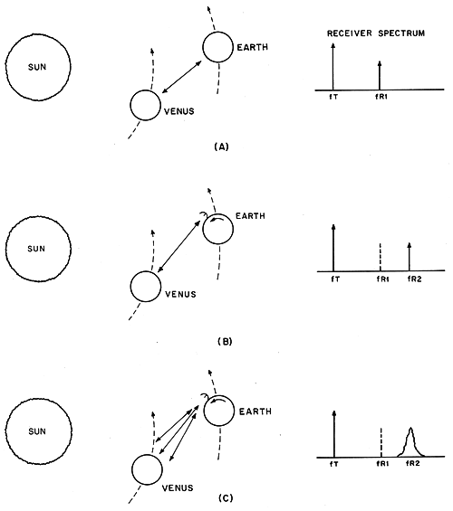
Doppler Shift Effects Although the radar equation gives the total power we expect to be returned from a target, it tells us nothing about how that power is distributed in frequency. Because our target is moving relative to Earth, the echo will not appear at the transmitted frequency; in fact, for Venus the echo frequency will not even be constant. Relative motion of Earth and Venus causes a shift, fD, of - 2V / λ where V = velocity between the two bodies measured along the Earth-Venus line (see Fig. 1A). We adopt the convention that negative values of V mean that the two bodies are approaching each other; in this case the echo will be slightly higher in frequency than the transmitted wave (fD is positive). In addition to gross planetary motion, we must also include planetary rotation in predicting Doppler shifts. Because Earth spins on its axis, there will be a velocity component either toward or away from Venus of up to 400 m/s, owing to motion of the station resulting from the rotation. When Venus appears to be rising in the eastern sky, the station is moving toward the planet and the echo will be slightly higher in frequency; when Venus appears to be setting, the station is moving away and the frequency will be lower. But Venus also rotates, albeit slowly, so that the response from the approaching part of the planet will be at a higher frequency than the response from the receding part (Fig. 1C). If we transmit a continuous carrier, it will be reflected as a smeared (or broadened) replica of the original because of the different amounts of Doppler shift imparted by various parts of the target. As if the Doppler shifts and spreadings were not annoying enough, we should also note that they all vary with time. The Doppler spreading caused by rotation of Venus does not vary much during the course of a day, but the shifts can change drastically. The solar system is on such a large scale that we often forget that the planets are quite literally hurtling through space, by terrestrial standards. For exam- pie, on July 1, 1978, Earth was traveling at over 30 km/s. At the same time, Venus was approaching at a relative velocity of more than 12 km/s. Of course we didn’t collide because the trajectories of the two planets are ellipses which do not intersect, but Earth and Venus do pass within 40 million kilometers from time to time. In 1978, this “inferior conjunction” occurred on November 9. At conjunction, the Doppler shift passes from positive through zero to negative, and the planets then drift apart. During the 24-hour period around the time of closest approach, the Doppler shifts from gross planetary motion will change by about 1000/λ Hz; Earth rotation superimposes another 1600/λ Hz shift between Venus rise and Venus set. The echo, which is only a few hertz wide, can best be detected with the aid of a narrow-bandwidth receiver. However, because the signal is constantly drifting, the passband must be constantly relocated. This combination of narrow bandwidth and accurate tuning is a challenging hardware requirement for today’s radio amateur. Let’s discuss the implications of these challenges. Prospects In this final section we consider the requirements for detecting a Venus echo and match the requirements against capabilities of state-of-the-art equipment. Not all of this equipment is within range of a typical radio amateur’s budget. The possibility exists, however, that enough of it could be assembled by a team of technically adept amateurs, and the feat accomplished within a few years. First consider the radar equation. At its closest approach on November 9, Venus was at a distance R of approximately 4.0 x 10¹⁰ meters from Earth. From astronomical studies, the radar cross section of Venus is known to be in the neighborhood of 10 percent of its disk area, or σ = 1013 m2 (the radius of Venus is about 6100 km). If we have a parabolic antenna 10 m in diameter, this gives us a geometrical area of about 80 m2. Taking an efficiency factor of 50 percent, we’re left with 40 m2 for reception. The gain-to-area rule of thumb translates this to 45 dB gain at 2300 MHz. If we assume the transmitter final amplifier power input is 1000 watts and its efficiency is also 50 percent, PT = 500 watts. From these values the radar equation allows us to compute the expected received power, PR = (500) (1013) (40)2 / 4π (4.0 x 10¹⁰) 4 (0.13)2 = 1.5 x 10⁻²³ watts Because Venus rotates, this power is spread over approximately 4 Hz under typical conditions, leaving us with 4.0 x 10⁻²⁴ watts/Hz power density in the received spectrum. This isn’t much, but under good conditions it might be distinguished from the background noise. Noise power which appears at the output of a receiver system arises from two principal sources. First are the natural emissions of the target and of the deep space background. Venus has a surface temperature on the order of 800°K (1000°F), which makes it an important source of microwave energy. The planet occupies such a small portion of the beamwidth of the 10 meter diameter antenna, however, that its radiation is effectively lost in the much colder background and it may be neglected here. When Venus is closest to Earth, it will be viewed against a background of maximum solar radiation, however, decreasing the possibilities for success of this experiment. Observations earlier or later than inferior conjunction will move the planet away from the sun and result in less solar noise but at the cost of increased range, which enters the radar equation as R4. The critical factors for determining optimum observation dates will be the beam pattern and distribution of solar noise across the sky. These can be obtained on a station by station basis and the results evaluated in terms of the EVE problem. For the remainder of this article we will assume that solar noise is not a problem. In practice, however, the probability for detection based on the conditions given here would have to be reduced somewhat. The second source of noise is the receiving system itself, and for 2300 MHz work is more important than natural noise. Microwave maser front ends are capable of equivalent noise temperatures less than 25 °K; we will assume that the receiver available for amateur work is not quite this good say T = 50°K, which corresponds to a noise figure of about 0.7 dB. The noise power, PN, produced can then be computed from the simple equation PN = kTB where k = Boltzmann’s constant (1.38 x 10⁻²³) watt-seconds/°K and B = receiving system bandwidth For the sake of simplicity, we will keep things on a per-unit bandwidth basis and set B = 1 Hz. The 50°K system then has a noise-power density of about 7.0 x 10⁻²² W/Hz, or about 175 times that of our hypothetical echo ! Readers who have trouble reading S5 signals on 40 meters may detect a problem lurking here. This is where the story of the Doppler drifts comes in. It is possible to take recordings of a large number of signals buried in noise and average them together to improve overall signal to noise ratio, if the signal is the same in each case. This may be done in either the time or frequency domain. Since we are already working with W/Hz, we’ll continue to use the latter and assume that some kind of spectrum analyzer is available to be attached to the receiver output. If the noise characteristics of each echo are the same (in a probabilistic sense), the random fluctuations will tend to cancel out when they are averaged, and the deterministic components of the signal will begin to peak through. Probability theory tells us that if N is the number of averages performed, the random fluctuations die out as N1/2. If we want our Venus echo to have approximately a 50 percent chance of being detected in the noise, we must boost its prominence by a factor of about 175, or average together about 30,000 signals. If we obtain one spectrum each second from the analyzer, over eight hours of data are required. Under normal circumstances, several days would be needed to accumulate this much data. Over an eight-hour period, the echo will solar noise have drifted a considerable amount, so it is important that tuning to compensate for Doppler shifts be accurate. Otherwise, the echoes will be averaged with noise, instead of with each other. The easiest solution to the tuning problem is to use a programmable local oscillator in the receiver; its frequency could be controlled by a small computer operating on predictions available from any number of sources. The computer might also be able to handle the spectral analysis and averaging, leaving the operator to monitor and control the transmitter and antenna. This combination of 10 meter diameter parabolas, kilowatt 2300 MHz transmitters, narrowband receivers with 50°K equivalent noise temperatures, and small computers operating programmable local oscillators is not to be found in every ham’s garage. Receiver front-end components with noise figures in the 1,5 dB range are available in the $100 price class and single-digital ICs are obtainable to perform the spectral analysis. The practical problems associated with signal detection, such as insuring that both transmitter and receiver frequencies are accurate to at least 1 Hz over periods of several days, are imposing enough that even the equipment described here would probably be. insufficient to obtain echo detection. It is likely that those who obtain the first echoes from Venus will find short cuts through the radar-equation calculations given in this article - using a shorter wavelength might have some advantage, for example. Use of a larger antenna would lead to an immediate improvement in signal-to-noise ratio. Though the task will never be easy, there are now individuals in the amateur ranks with the necessary expertise to work EVE. The prospects for two-way communication (with exchange of signal reports) are quite discouraging, but successful detection of the echo itself sometime in the not- too-distant future should not come as a complete surprise. Acknowledgements The helpful suggestions supplied by W1XZ, W6HD, K6HWJ and WA6VBA during preparation of this article were appreciated. QST December 1978 Made by OK1TEH for OK2KKW.com pages - 2008 |