Smith chart and a design of asymmetrical power divider

After publication of this small article I’m target of ham radio collegues, who are asking for design of some unsymetric splitter for drive of two (or more) PAs. So, maybe will be more effective such design describe into details and teach them. I don’t know why, but between ham radio ops still exists some shyness to the design of matching circuits by Smith chart. Let’s look deeper:

For 2014 UHF Contest we needed drive power for DH5FS’s PA. As he asked for, this PA request for full PWR about 4W drive, however our old GS31 brick 10x more. So, it was necessary to produce splitter 90/10%, which will be able hold some 45W on the input and distribute it in the ratio 40 and 4W into two outputs.

How to do it?

At first – any design of power splitter presumes, that on the input as well as all outputs will be connected devices with REAL IMPEDANCE 50 Ω! Without good covering of such obligation the splitter will never works well! Beside other troubles, like change of splitting ratio in case of use of different cable lengths, the requested ratio will never be correct and one PA could be overloaded and the next one not fully loaded. To ensure such proper duty the connected PAs must be very well matched to 50Ω without any capacitive, or inductance complex part of inductance. Block schematics of such splitter will be like this one:

To be able design such matching circuits, is needed to know value of impedance Z1 and Z2. But, of course, the impedance Z1 and Z2 must be complementary to get 50 Ω by parallel connection of both matching circuits. And this condition is a swell as the key for correct splitting ratio – in such case 90 and 10% of input power. Let’s remind to the secondary school physics: Kirchhof law says, that the summ of currents flowing into the node are equal to the summ of currents from the node flowing out. Clear isn’t it?

For calculation let’s put some virtual input power, for example 100W (100%). In case of such power will be voltage on 50 Ω input of splitter:

U = root of (100*50) = 70.7 V  and the RF current flowing into a splitter will be: I = P/R = 1.41 A

If we want to split the input power in the ratio 90 / 10%, in the same ratio must be distributed the currents, flowing into these matching circuits: it mean into input of first match the current will be 1.41*0.9 and into the second 1.41*0.1 A… it mean 1.27 A and 0.41 Amps! And because the voltage there is the same (it’s one circuit node),  we already can calculate input impedances of these matching “boxes”:

Z1  = U / I = 70.7 / 1.27 = 55.7 Ω     and     Z2 = 70.7 / 0.14 = 501 Ω

For verification let’s calculate parallel combination of 55.7 and 501 Ω (it should be 50 Ω again) and we can see, that the result is 50.1 Ω! It mean, verification passed! :-)

The input for matching boxes design is that:

Now we have the second part of task – to design such matching circuits, which will be able match the input impedance  on dedicated operation frequency (in such case 432MHz)  to the 50 Ω output impedance!

Probably the best way is use of Smith chart. Most simple way is do the graphic task on PC: download the Smith chart – for example here or here.

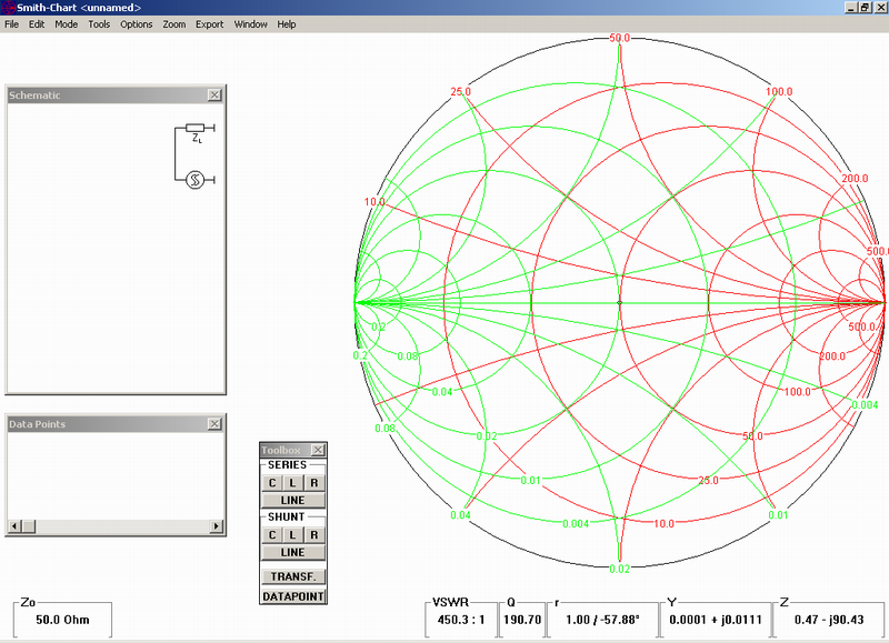
When the SW is running you will see the picture, like this one:

However, this picture is a little bit confusing – but simple click on “options” and delete the “Y-chart” The picture became much more “user friendly”:

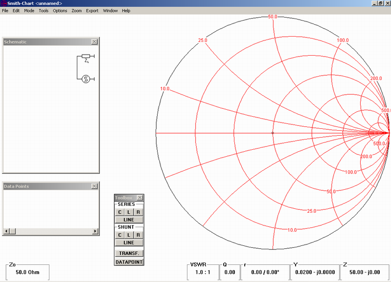
In the box bottom left is the value of normalized impedance of the Smith chart. Default level is a 50Ω, but it could be changed. This value correspond to the center of circle of Smith chart on right side. Now you can move by mouse the cursor to the center and you will see, that the impedance there is really 50 Ω without any imaginary (complex) part of impedance (capacitive, or inductive) , which is assigned by letter “j” In horizontal line the impedance is changing from the zero (on left) to infinity (right). When the cursor will be moved to the upper half of the circle, we will move through area of inductive impedance part (inductance), if move to the bottom, there is a capacitive area of impedance (capacitance). Capacitance has negative sign! Test it please!

And now to the real task: we are asked to match (in our case) 501 Ω real impedance to the 50 Ω. In both cases it is just real impedance without any complex (inductive, or capacitive part).

• now in the “toolbox” of the cart SW open the dialog box “datapoint” and insert requested data. Matching we will calculate from the side of 501 Ω  in direction to the 50 Ω load. Put the 501 Ω value to the “toolbox” and into the imaginary part put the zero. It defines in the Smith chart the point of input impedance – see the chart:

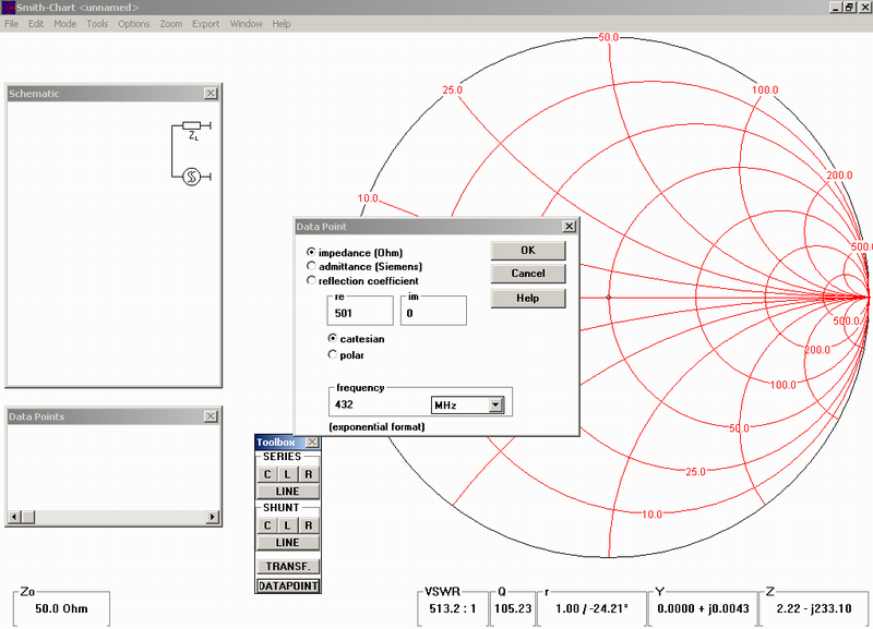
When you confirm this task by click on, you’ll see the point on the chart, assigned as “1” on the place, where the circle 500 Ω crossing horizontal line of zero complex impedance (admitance is the common name for both imaginary part of impedance – capacitance and an inductance). Now you have for choice, how to make next step. Let’s use the “toolbox” again. Always you have lot of options. Even the simpliest – move from 501 Ω to 50 Ω by series resistor 451 Ω hi… But we need transfer impedance without losses. The optimal way is used combination of capacitors and inductors (coils), like on HF bands popular “Pi circuit” in the antenna box, or even (particularly on VHF and UHF bands) part of lines (mostly coaxial or microstrip)  for loss free transformation. In such case select such way, where you will avoid very small inductance and capacitance to prevent influence of parazitics capacity of coils and inductance of capacitors connection, because these additional transformations may shame the whole design.  For selection of type of the device and a connection into a circuit use left button on your mouse and the right one help you go one step back in case of wrong selection. For our task – when the use of resistors and transformers will be avoided, you have for possible use for example these options:

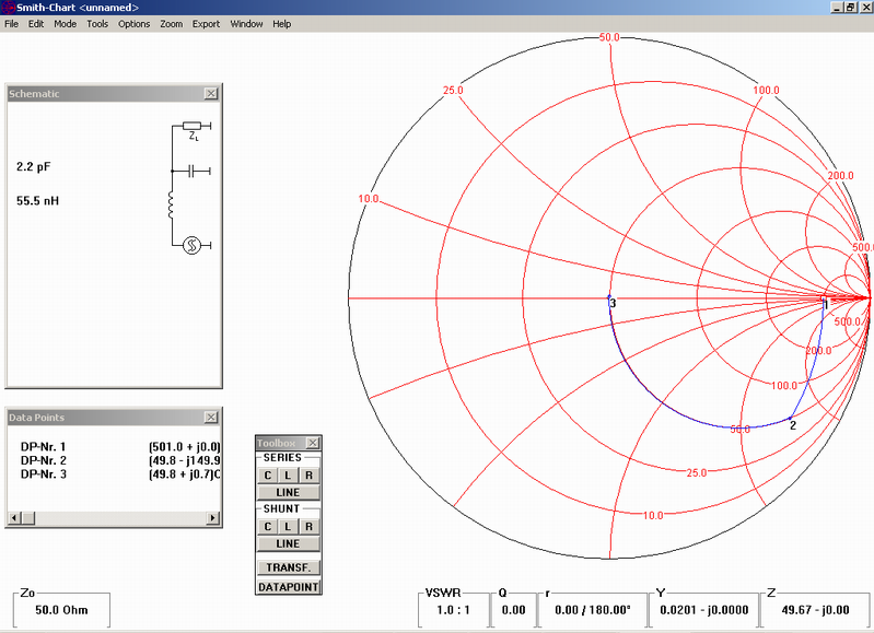
a)      parallel capacitor 2.2pF and a series coil with inductance 55.5nH:

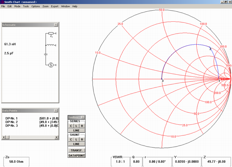
b) parallel coil 61.3nH and a capacitor 2.5pF in series:

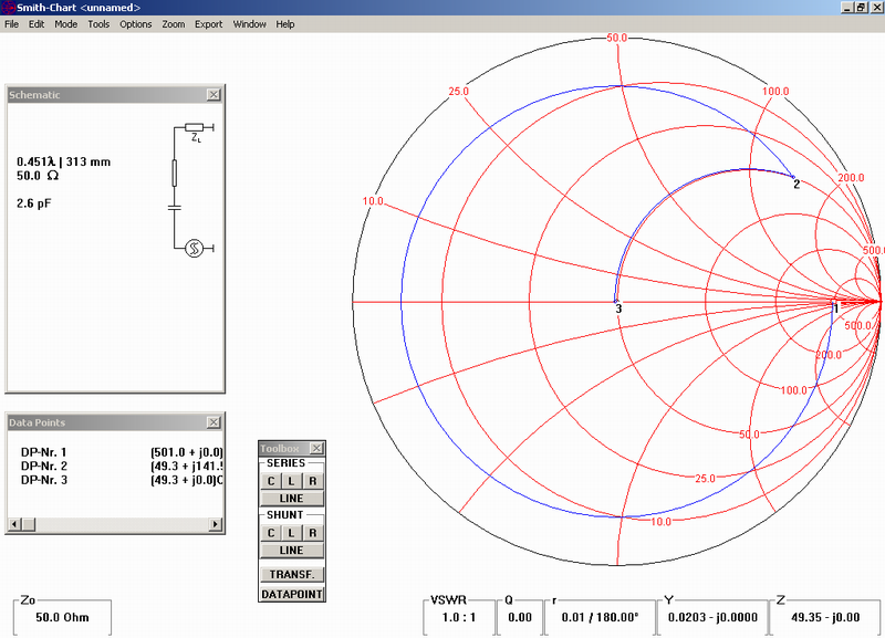
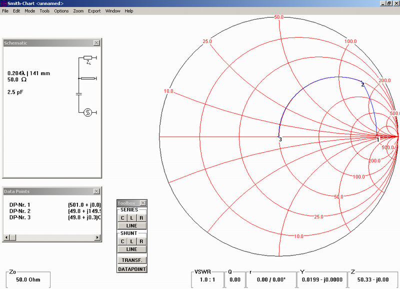
c)   coaxial line with impedance 50 Ω (for example semirigid cable) with length 0.451 lambda in series and a capacitor 2.6pF in series:

d)      parallel, on the end short connected coaxial cable 50 Ω, 0.21 lambda long  and a capacitor 2.5pF in the series:

Based on different tasks of course may exists plenty different combination of matching lines, but because the basic law says, that “you can’t band the physics”, all of these solutions must be visible inside the circle of Smith chart, which is truly ingenious invention, worthy to Nobel price in electronics. P.H.Smith his "Smith chart" released in the August 1958 and he has succeeded in one chart by the graphic way demonstrate all mathematic relations not only between impedances and admitances, but as well as many other mathematic tasks of electronic circuits design – like areas of stability for amplifiers and oscillators…

BTW: if you will want to use such chart for example for design of tube amplifier (for example with GS35 tube), so this tube will have with full power drive on the anode (in case of B class) real part of impedance about 2 kΩ  and some capacity between anode and grid and anode to ground, in sum abt. 5.5pF The anode circuit for 70cm band you can model on the Smith chart for example this way:

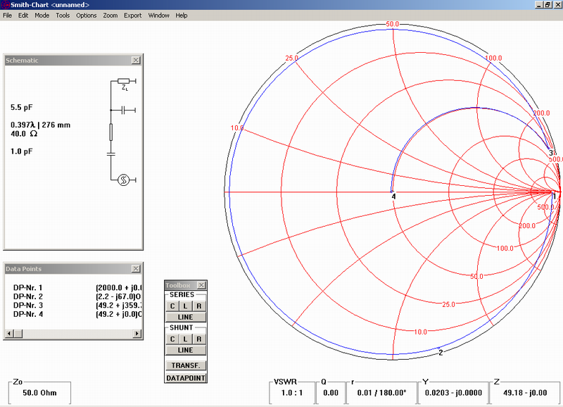
The result (without influence of tuning capacitor) you can compare with real construction for example here. The input impedance of the tube has the real part is 1/steepness (mA/V) and for such tube will be somewhere abt. 25 Ω and a cathode to grid capacity you will find in the datasheet… Simple,  isn’t it?

But back to our task: matching circuit from 501 to 50 Ω could be realized by series combination of coaxial line 0.451 lambda with capacitor 2.6pF. Due to velocity of teflon dielectric of a semirigid cable (0.7) the physical length of cable will be abt. 22cm and a series capacity 2.7pF.

Similarly the 55.7 Ω to 50 Ω matching circuit we can setup from 18.4cm long semirigid and 68pF capacitor in series. Confirm it on your Smith chart SW in the PC!  In case of design works close to 50 Ω use the zoom tool.  Such design is much easier, that you may expect!

However – because across coupling capacitor 68pF is transferring quite high power (40W) would be good idea to verify, if such capacitor will not burn out in operation: we would intent to use “standard” ceramic capacitor 68pF/500V made from low loss NPO ceramics, for example this one (http://www.gmelectronic.com/ck-68p-500v-npo-gym-rm5-08-5-p120-024). The capacitor producer declares for it the Q at least 1000 – see here. The quality (Q) of capacitor is de facto upside-down value of his dielectric loss factor (tangent delta). See here.  It mean, that from the Q of capacitor and a frequency we can calculate serial dissipation resistance of capacitor (ESR):

ESR = 1/ Q*(2PI*f*C) = 1/ 1000*(6,28*432e6*75e-12) = 4,9 miliohm

In case of 40W the RF current passing through of this capacitor will be 0.853A, so the power (thermal) lost in capacitor will be P = R*I²  = 0.0049*0.853*0.853 = 3.5mW. Such small power should not make any problem for the capacitor, because this thermal power could be easy radiated away. This capacitor is then OK for such use. However – for another similar use and particularly for higher power would be sometime needed to use capacitors with higher Q – for example MICA capacitors, and/or special low loss ceramics capacitors, well known from SSPAs (here, here).

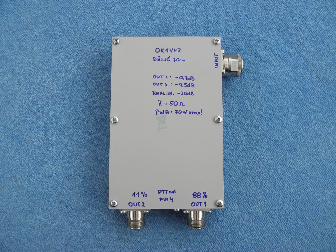
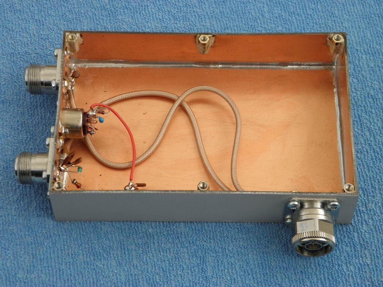
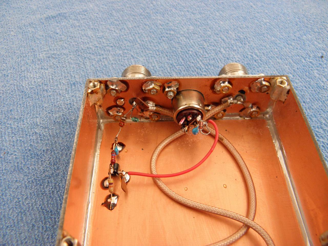
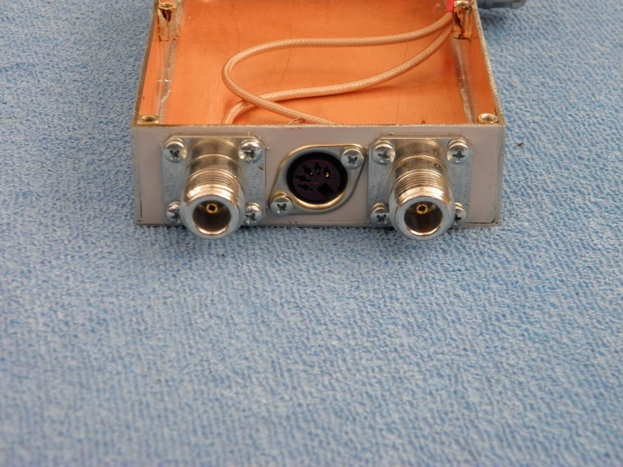
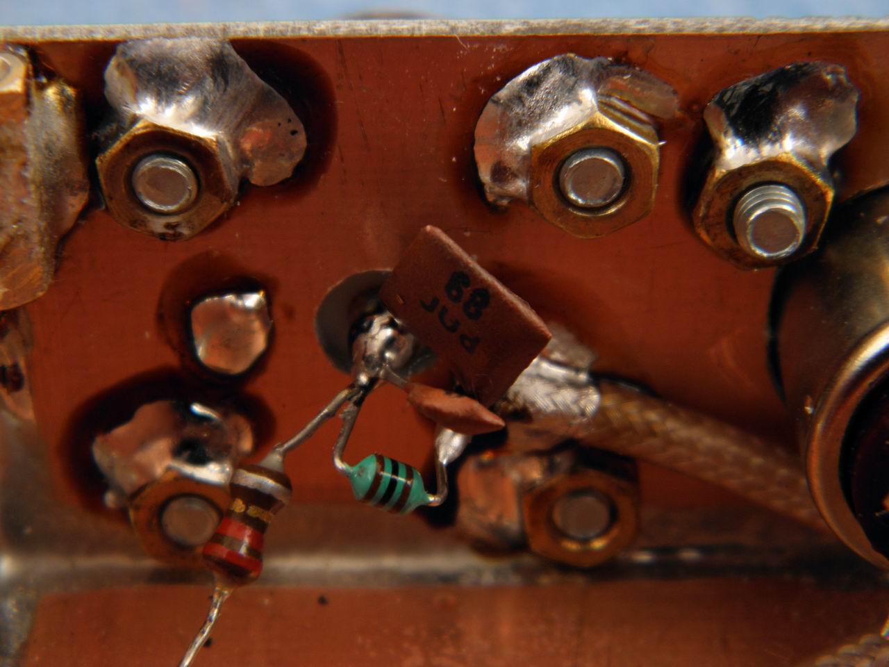
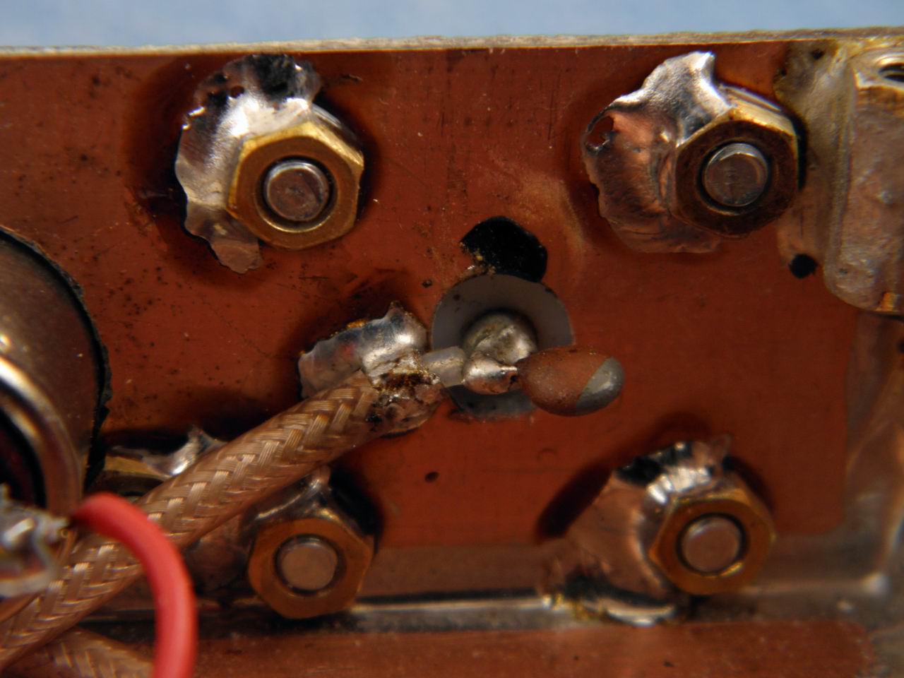
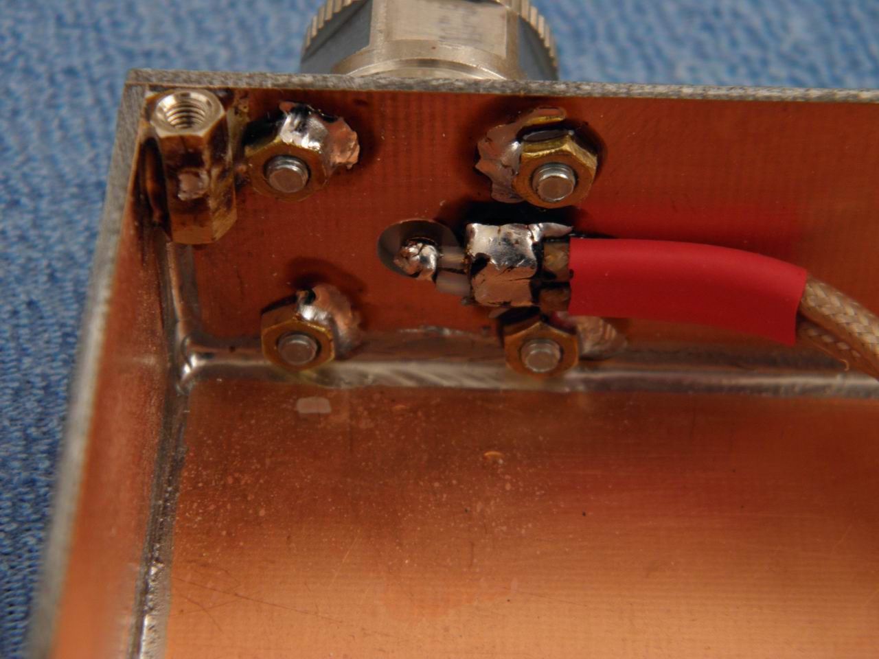
Theoretically we have the splitter design ready for construction. Just for idea, here are pictures of my solution – the box is made from PCB boards and on the top of above RF design consist of  the FET switch for PTT over the coax and a choke parallel to 68pF capacitor for transfer of DC for PTT to the connected PA. All of the connections are in the “UHF style”.

When you are looking to develop something similar and use for a design the Smith chart, it will be for sure good help for final success. But don’t forget, that such RF device must be terminated correctly on all ports! If the output termination will be not right, the splitting factor will be always some-how different, than the designed one!

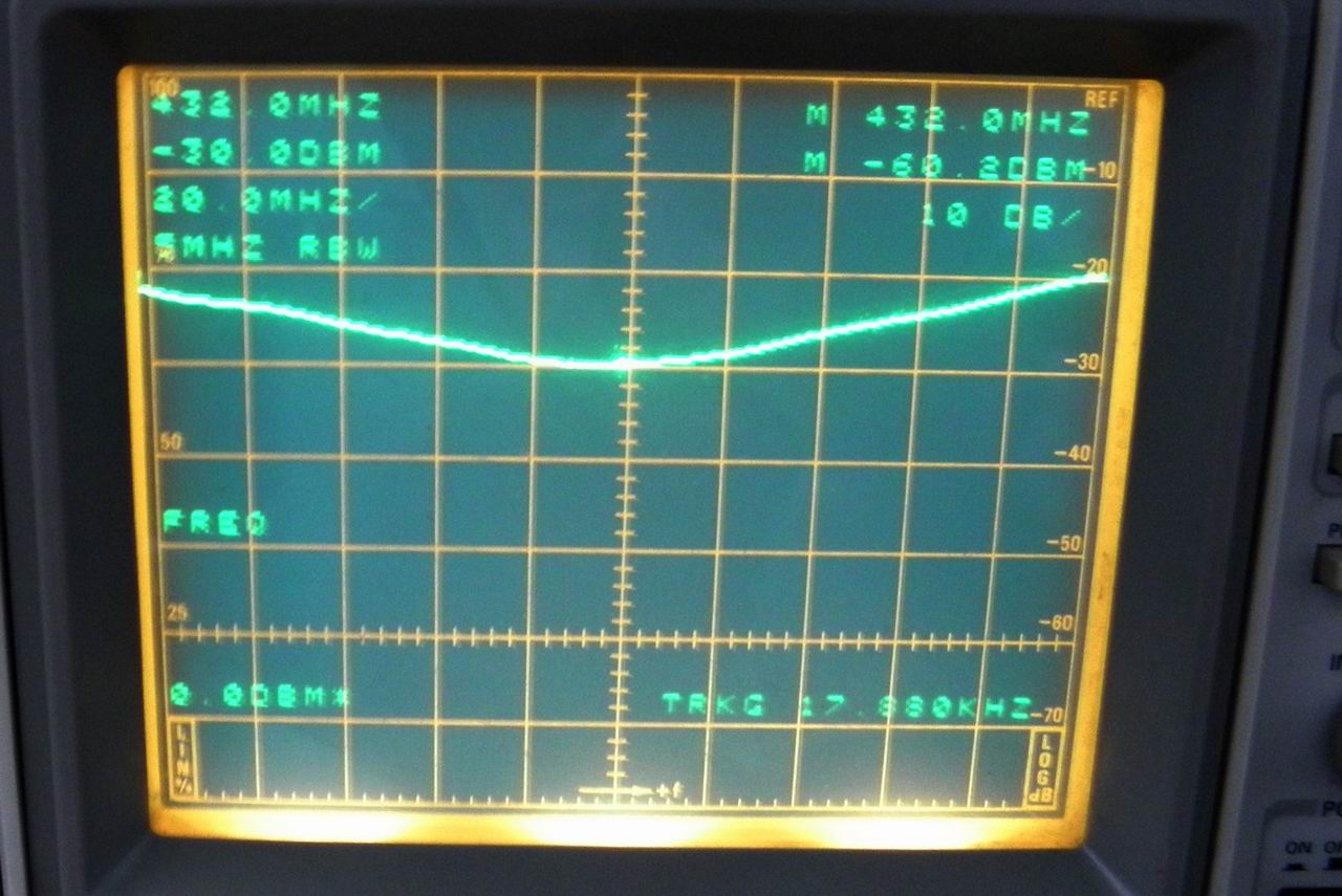
For final: check the constructed splitter for performance. Of course nothing is perfect! In my sample I got the input attenuation of reflection about 20dB (SWR abt. 1:1.2) and the splitting factor is 88 / 11 %. It is acceptable precision in ham radio conditions. 

But – and it is natural – such splitter can not be used in opposite direction! When you terminate the input and one output port and start to measure reflections on the other output port (particularly the 10% port), the results must be bad. Why? It’s simple:  such divider cannot be reciprocal!  The matching circuit for 10% output port transform input impedance from 501 to 50 Ω. And opposite, from perspective (from the direction looking back into the 10% output port) of output, 50 to 501 Ω. But the 501 Ω point is connected in such case to the point, where is parallel connection of input 50 Ω terminator and abt. 55.7 Ω impedance from the other (as well as terminated) output port (90%). So, parallel connection of 50 and 55.7 Ω give you some 26 Ω. It is more, than clear, that 501 Ω impedance, tranformed  from the tested 10% output, cannot be matched! So – such power divider design cannot be used opposite way as a matched power combiner! However – if you will need something like it, with your experience, gave in the above design test, you will do it! Smith chart is reliable tool for such games, hi.

73 de OK1VPZ

and a few pics (click on for full size)